
- 참고 : 핸즈온 머신러닝 2판
텐서플로를 사용한 사용자 정의 모델과 훈련
- 자신만의 손실 함수, 지표, 층, 모델, 초기화, 규제, 가중치 규제 등을 만들어 세부적으로 제어하고 싶을 때 필요
- 텐서플로의 자동 그래프 생성 기능을 사용해 사용자 정의 모델과 훈련 알고리즘의 성능을 향상 시킬수 있는 방법
텐서플로 훝어보기
이미지 분류, 자연어 처리, 추천 시스템, 시계열 예측 등과 같은 모든 종류의 머신러닝 작업 수행
tensorflow 구성 이미지
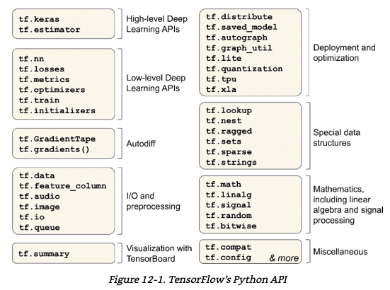
- 가장 저수준의 tensorflow 연산은 매우 효율적인 C++ 코드로 구현
대부분의 코드는 고수준 API를 사용, 하지만 더 높은 자유도가 필요하는 경우 저 수준 API를 사용해 직접 텐서를 처리
numpy처럼 텐서플로 사용하기
텐서와 연산
- tf.constant() 함수로 텐서를 생성 할수 있음
- ndarray와 마찬가지로 tf.Tensor는 크기와 데이터 타입(dtype)을 가짐
tf.constant([[1., 2., 3.], [4., 5., 6.]]) # 행렬
tf.constant(42) # 스칼라

t.shape
>> TensorShape([2, 3])
t.dtype
>> tf.float32
- index 참조도 numpy와 유사
- tf.newaxis 는 차원을 하나 추가하는 것 (tf.expand_dims 와 유사)
t[:, 1:]
>> <tf.Tensor: shape=(2, 2), dtype=float32, numpy=
    array([[2., 3.],
           [5., 6.]], dtype=float32)>

t[..., 1, tf.newaxis]
>> <tf.Tensor: shape=(2, 1), dtype=float32, numpy=
    array([[2.],
           [5.]], dtype=float32)>
- 모든 종류의 텐서 연산이 가능함
- tf.square 은 제곱을 계산
t + 10
>> <tf.Tensor: shape=(2, 3), dtype=float32, numpy=
    array([[11., 12., 13.],
           [14., 15., 16.]], dtype=float32)>

tf.square(t)
>> <tf.Tensor: shape=(2, 3), dtype=float32, numpy=
    array([[ 1.,  4.,  9.],
           [16., 25., 36.]], dtype=float32)>

t @ tf.transpose(t) # (2,3) 행렬곱 (3,2) 결과
>> <tf.Tensor: shape=(2, 2), dtype=float32, numpy=
    array([[14., 32.],
           [32., 77.]], dtype=float32)>
텐서와 넘파이
- 텐서는 넘파이와 함께 사용하기 편리함
- 넘파이 배열로 텐서를 만들 수 있고 그 반대도 가능
- 넘파이 배열에 텐서플로 연산을 적용할 수 있고 텐서에 넘파이 연산을 적용할 수도 있음
a = np.array([2., 4., 5.])
tf.constant(a)
>> <tf.Tensor: shape=(3,), dtype=float64, numpy=array([2., 4., 5.])>

t.numpy()
>> array([[1., 2., 3.],
       [4., 5., 6.]], dtype=float32)

tf.square(a)
>> <tf.Tensor: shape=(3,), dtype=float64, numpy=array([ 4., 16., 25.])>

np.square(t)
>> array([[ 1.,  4.,  9.],
       [16., 25., 36.]], dtype=float32)
타입 변환
- 타입 변환은 성능을 크게 감소시킬 수 있음
- tensorflow는 어떤 타입 변환도 자동으로 수행하지 않음
- 호환되지 않은 타입의 텐서로 연산을 실행하면 예외가 발생
- 실수와 정수 텐서는 연산이 불가능
- type 변환시는 tf.cast() 사용
t2 = tf.constant(40., dtype=tf.float64)
tf.constant(2.0) + tf.cast(t2, tf.float32)
>> <tf.Tensor: shape=(), dtype=float32, numpy=42.0>
변수
tf.Tensor는 변경이 불가능한 객체
일반적인 텐서로는 역전파로 변경되어야 하는 신경망의 가중치를 구현할 수 없음
시간에 따라 변경되어야 할 다른 파라미터도 존재
이를 위해서 tf.Variable이 필요
tf.variable은 tf.tensor와 비슷하게 동작, 동일한 연산을 수행할 수 있고 넘파이와 호환이 좋음
assign() 메서드를 통해 변수값 변경이 가능 (assign_add, assign_sub를 통해 주어진 값만큼 변수 증감 가능)
slide + assign , scatter_update(), scatter_nd_update() 메서드를 사용해 개별 원소 수정
v = tf.Variable([[1., 2., 3.], [4., 5., 6.]])
v.assign(2 * v)
>> [[ 2.,  4.,  6.],[ 8., 10., 12.]]

v[0, 1].assign(42)
>> [[ 2., 42.,  6.], [ 8., 10., 12.]]

v[:, 2].assign([0., 1.])
>> [[ 2., 42.,  0.], [ 8., 10.,  1.]]
다른 데이터 구조
- 희소 텐서 (tf.SparseTensor)
- 대부분 0으로 채워진 텐서를 효율적으로 나타냄, tf.sparse 패키지는 희소 텐서를 위한 연산을 제공
- 텐서 배열 (tf.TensorArray)
- 텐서의 리스트, 기본적으로 고정된 길이를 가지지만 동적으로 변경가능, 리스트에 포함된 모든 텐서는 크기와 데이터 타입이 동일해야 함
- 래그드 텐서(tf.RaggedTensor)
- 리스트의 리스트에 해당, 텐서에 포함된 값은 동일한 데이터 타입을 가져야 하지만 리스트의 길이는 다를 수 있음
- 문자열 텐서(tf.string)
- 집합(tf.sets)
- 일반적인 텐서로 표현, tf.sets를 통해 연산을 사용가능
- 큐
- 단계별로 텐서를 저장, 여러 종류의 큐를 제공
사용자 정의 모델과 훈련 알고리즘
사용자 정의 손실 함수
희귀 모델을 훈련하는 데 훈련 세트에 잡음 데이터가 조금 있다고 가정시 이상치를 제거하거나 고쳐서 데이터셋을 수정할수 있지만 비효율적
사용자 맞춤으로 손실을 정의할 수 있음
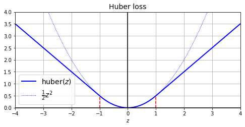
Huber loss 구현예제
from sklearn.datasets import fetch_california_housing
from sklearn.model_selection import train_test_split
from sklearn.preprocessing import StandardScaler

housing = fetch_california_housing()
X_train_full, X_test, y_train_full, y_test = train_test_split(
    housing.data, housing.target.reshape(-1, 1), random_state=42)
X_train, X_valid, y_train, y_valid = train_test_split(
    X_train_full, y_train_full, random_state=42)

scaler = StandardScaler()
X_train_scaled = scaler.fit_transform(X_train)
X_valid_scaled = scaler.transform(X_valid)
X_test_scaled = scaler.transform(X_test)
def huber_fn(y_true, y_pred):
error = y_true - y_pred
is_small_error = tf.abs(error) < 1
squared_loss = tf.square(error) / 2
linear_loss = tf.abs(error) - 0.5
return tf.where(is_small_error, squared_loss, linear_loss)
plt.figure(figsize=(8, 3.5))
z = np.linspace(-4, 4, 200)
plt.plot(z, huber_fn(0, z), "b-", linewidth=2, label="huber($z$)")
plt.plot(z, z**2 / 2, "b:", linewidth=1, label=r"$\frac{1}{2}z^2$")
plt.plot([-1, -1], [0, huber_fn(0., -1.)], "r--")
plt.plot([1, 1], [0, huber_fn(0., 1.)], "r--")
plt.gca().axhline(y=0, color='k')
plt.gca().axvline(x=0, color='k')
plt.axis([-4, 4, 0, 4])
plt.grid(True)
plt.xlabel("$z$")
plt.legend(fontsize=14)
plt.title("Huber loss", fontsize=14)
plt.show()
사용자 정의 요소를 가진 모델을 저장하고 로드하기
- 사용자 정의 객체를 포함한 모델을 로드할때는 해당 객체를 매핑해야 함
model.save("my_model_with_a_custom_loss.h5")
model = keras.models.load_model("my_model_with_a_custom_loss.h5",
                                custom_objects={"huber_fn": huber_fn})
model.fit(X_train_scaled, y_train, epochs=2,
validation_data=(X_valid_scaled, y_valid))- 매개변수를 받는 huber_fn
def create_huber(threshold=1.0):
    def huber_fn(y_true, y_pred):
        error = y_true - y_pred
        is_small_error = tf.abs(error) < threshold
        squared_loss = tf.square(error) / 2
        linear_loss  = threshold * tf.abs(error) - threshold**2 / 2
        return tf.where(is_small_error, squared_loss, linear_loss)
    return huber_fn


model.compile(loss=create_huber(2.0), optimizer="nadam", metrics=["mae"])
model.fit(X_train_scaled, y_train, epochs=2,
          validation_data=(X_valid_scaled, y_valid))

model.save("my_model_with_a_custom_loss_threshold_2.h5")
model = keras.models.load_model("my_model_with_a_custom_loss_threshold_2.h5",
                                custom_objects={"huber_fn": create_huber(2.0)})

model.fit(X_train_scaled, y_train, epochs=2,
validation_data=(X_valid_scaled, y_valid))- keras.losses.Loss 클래스 상속하고 get_config() 매서드를 구현하는 방식으로 구현
class HuberLoss(keras.losses.Loss):
    def __init__(self, threshold=1.0, **kwargs):
        self.threshold = threshold
        super().__init__(**kwargs)
    def call(self, y_true, y_pred):
        error = y_true - y_pred
        is_small_error = tf.abs(error) < self.threshold
        squared_loss = tf.square(error) / 2
        linear_loss  = self.threshold * tf.abs(error) - self.threshold**2 / 2
        return tf.where(is_small_error, squared_loss, linear_loss)
    def get_config(self):
        base_config = super().get_config()
        return {**base_config, "threshold": self.threshold}


model = keras.models.Sequential([
    keras.layers.Dense(30, activation="selu", kernel_initializer="lecun_normal",
                       input_shape=input_shape),
    keras.layers.Dense(1),
])- 모델을 컴파일 할때 이 클래스의 인스턴스 사용 가능
- 모델을 저장할 때 임계값도 같이 저장됨, 모델을 로드할 때 클래스 이름과 클래스 자체를 매핑해야 함
model.compile(loss=HuberLoss(2.), optimizer="nadam", metrics=["mae"])
model.fit(X_train_scaled, y_train, epochs=2,
          validation_data=(X_valid_scaled, y_valid))

model.save("my_model_with_a_custom_loss_class.h5")
model = keras.models.load_model("my_model_with_a_custom_loss_class.h5",
                                custom_objects={"HuberLoss": HuberLoss})
model.fit(X_train_scaled, y_train, epochs=2,
          validation_data=(X_valid_scaled, y_valid))
활성화 함수, 초기화, 규제, 제한을 커스터마이징하기
- 사용자 정의 함수 예시
# 사용자 정의 tf.nn.softplus(z)
def my_softplus(z): # tf.nn.softplus(z) 값을 반환합니다
    return tf.math.log(tf.exp(z) + 1.0)

# 사용자 정의 글로럿 초기화
def my_glorot_initializer(shape, dtype=tf.float32):
    stddev = tf.sqrt(2. / (shape[0] + shape[1]))
    return tf.random.normal(shape, stddev=stddev, dtype=dtype)

# 사용자 정의 L1 규제
def my_l1_regularizer(weights):
    return tf.reduce_sum(tf.abs(0.01 * weights))

# tf.nn.relu(weight)와 반환값이 같음
def my_positive_weights(weights): # tf.nn.relu(weights) 값을 반환합니다
return tf.where(weights < 0., tf.zeros_like(weights), weights)- 사용자 정의 함수에 따라서 매개변수가 달라짐, 만들어진 사용자 정의 함수는 보통의 함수와 동일하게 사용할 수 있음
- 아래 예시에서 Dense 층에 가중치 초기화, 규제등 함수를 적용할수 있음
layer = keras.layers.Dense(1, activation=my_softplus,
                           kernel_initializer=my_glorot_initializer,
                           kernel_regularizer=my_l1_regularizer,
                           kernel_constraint=my_positive_weights)

model.save("my_model_with_many_custom_parts.h5")
model = keras.models.load_model(
    "my_model_with_many_custom_parts.h5",
    custom_objects={
       "my_l1_regularizer": my_l1_regularizer,
       "my_positive_weights": my_positive_weights,
       "my_glorot_initializer": my_glorot_initializer,
       "my_softplus": my_softplus,
})- 함수가 모델과 함께 저장해야 할 파라미터를 가지고 있다면 keras.regularizers.Regularizer, keras.constraints.Constraint, keras.initializers.Initializer, keras.layers.Layer와 같이 적절한 클래스를 상속
class MyL1Regularizer(keras.regularizers.Regularizer):
    def __init__(self, factor):
        self.factor = factor
    def __call__(self, weights):
        return tf.reduce_sum(tf.abs(self.factor * weights))
    def get_config(self):
        return {"factor": self.factor}

keras.backend.clear_session()
np.random.seed(42)
tf.random.set_seed(42)

model = keras.models.Sequential([
    keras.layers.Dense(30, activation="selu", kernel_initializer="lecun_normal",
                       input_shape=input_shape),
    keras.layers.Dense(1, activation=my_softplus,
                       kernel_regularizer=MyL1Regularizer(0.01),
                       kernel_constraint=my_positive_weights,
                       kernel_initializer=my_glorot_initializer),
])
사용자 정의 지표
- 손실과 지표는 개넘적으로 다른 것이 아님
- 손실은 모델을 훈련하기 위해 경사 하강법에서 사용하므로 미분 가능해야 하고 그래이디언트가 모든 곳에서 0이 아니어야 함
- 지표는 모델을 평가할때 사용, 미분이 가능하지 않거나 모든 곳에서 그레이디언트가 0이어도 됨
model = keras.models.Sequential([
    keras.layers.Dense(30, activation="selu", kernel_initializer="lecun_normal",
                       input_shape=input_shape),
    keras.layers.Dense(1),
])

model.compile(loss="mse", optimizer="nadam", metrics=[create_huber(2.0)])
model.fit(X_train_scaled, y_train, epochs=2)- 각 배치마다의 손실은 지표가 아님, 수학적으로는 손실 = 지표 * 샘플 가중치의 평균
- 이 때문에 지표를 통해 정확히 계산을 할수 있는 객체가 필요
- 아래와 같은 Precision() 객체는 batch마다 점진적 업데이트가 이루어지기 때문에 이를 스트리밍 지표라고 함
- result()를 호출하면 현재 지푯값을 얻을수 있음
- variables()를 사용해 변수 확인 가능
- reset_states()를 사용해 변수 초기화 가능
precision = keras.metrics.Precision()
precision([0, 1, 1, 1, 0, 1, 0, 1], [1, 1, 0, 1, 0, 1, 0, 1])
>> <tf.Tensor: shape=(), dtype=float32, numpy=0.8>
precision([0, 1, 0, 0, 1, 0, 1, 1], [1, 0, 1, 1, 0, 0, 0, 0])
>> <tf.Tensor: shape=(), dtype=float32, numpy=0.5>- 사용자 정의 스트리밍 지표
- keras.metrics.metric 클래스를 상속
- 전체 후버 손실과 지금까지 처리한 샘플 수를 기록하는 클래스, 결과값 요청시 평균 후버 손실 반환
class HuberMetric(keras.metrics.Metric):
    def __init__(self, threshold=1.0, **kwargs):
        super().__init__(**kwargs) # 기본 매개변수 처리 (예를 들면, dtype)
        self.threshold = threshold
        self.huber_fn = create_huber(threshold)
        self.total = self.add_weight("total", initializer="zeros")
        self.count = self.add_weight("count", initializer="zeros")
    def update_state(self, y_true, y_pred, sample_weight=None):
        metric = self.huber_fn(y_true, y_pred)
        self.total.assign_add(tf.reduce_sum(metric))
        self.count.assign_add(tf.cast(tf.size(y_true), tf.float32))
    def result(self):
        return self.total / self.count
    def get_config(self):
        base_config = super().get_config()
return {**base_config, "threshold": self.threshold}- 지표를 함수로 정의하면 앞서 수동으로 했던 것처럼 keras가 배치마다 자동으로 함수를 호출하고 에포크 동안 평균을 기록
- HuberMetric 클래스 정의하는 유일한 이점은 threshold를 저장하는 것
- 정밀도와 같이 어떤 지표는 배치에 걸쳐 단순히 평균을 낼 수 없음
- 해당 경우는 스트리밍 지표를 구현하는 것 외에 다른 방법이 없음
사용자 정의 층
- tensorflow에는 없는 특이한 층을 가진 네트워크를 만들어야 할 때
- keras.layers.Flatten, keras.layers.ReLU와 같은 층은 가중치가 없음
- 가중치가 필요 없는 사용자 정의 층을 만들기 위한 가장 간단한 방법은 파이썬 함수를 만든 후 keras.Layers.Lambda 층으로 감싸는 것
- 입력에 지수 함수를 적용하는 층
exponential_layer = keras.layers.Lambda(lambda x: tf.exp(x))

exponential_layer([-1., 0., 1.])
>> <tf.Tensor: shape=(3,), dtype=float32, numpy=array([0.36787948, 1.        , 2.7182817 ], dtype=float32)>
회귀 모델에서 예측값의 스케일이 매우 다를 때 출력층에 사용
- 가중치가 있는 층을 만들려면 keras.layers.Layer를 상속해야 함
- 여러 가지 입력을 받는 층을 만들때는 call() 메서드에 모든 입력이 포함된 튜플을 매개변수 값으로 전달
- 비슷하게 compute_output_shape() 메서드의 매개변수도 각 입력의 배치 크기를 담은 튜플이어야 함
- 여러 출력을 가진 층을 만들려면 call() 메서드가 출력의 리스트를 반환해야 함, compute_output_shape() 메서드는 배치 출력 크기의 리스트를 반환
- Dense층의 간소화 버전 예시
class MyDense(keras.layers.Layer):
    def __init__(self, units, activation=None, **kwargs):
        super().__init__(**kwargs)
        self.units = units
        self.activation = keras.activations.get(activation)

    def build(self, batch_input_shape):
        self.kernel = self.add_weight(
            name="kernel", shape=[batch_input_shape[-1], self.units],
            initializer="glorot_normal")
        self.bias = self.add_weight(
            name="bias", shape=[self.units], initializer="zeros")
        super().build(batch_input_shape) # must be at the end

    def call(self, X):
        return self.activation(X @ self.kernel + self.bias)

    def compute_output_shape(self, batch_input_shape):
        return tf.TensorShape(batch_input_shape.as_list()[:-1] + [self.units])

    def get_config(self):
        base_config = super().get_config()
        return {**base_config, "units": self.units,
"activation": keras.activations.serialize(self.activation)}- 두 개의 입력과 세 개의 출력을 만드는 층
class MyMultiLayer(keras.layers.Layer):
    def call(self, X):
        X1, X2 = X
        print("X1.shape: ", X1.shape ," X2.shape: ", X2.shape) # 사용자 정의 층 디버깅
        return X1 + X2, X1 * X2

    def compute_output_shape(self, batch_input_shape):
        batch_input_shape1, batch_input_shape2 = batch_input_shape
        return [batch_input_shape1, batch_input_shape2]

inputs1 = keras.layers.Input(shape=[2])
inputs2 = keras.layers.Input(shape=[2])
outputs1, outputs2 = MyMultiLayer()((inputs1, inputs2))
사용자 정의 모델
- 사용자 모델은 keras.model 클래스를 상속하여 층과 변수를 만들고 모델이 해야 할 작업을 call() 메서드에 구현
- 아래와 같은 모델을 만들 시
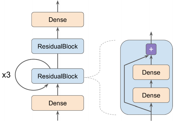
입력이 첫 번째 완전 연결 층을 통과하여 두 개의 완전 연결 층과 스킵 연결로 구성된 잔차 블록으로 전달
그 다음 동일한 잔차 블록에 세 번 더 통과시킴, 그 후 잔차 블록을 지나 마지막 출력이 완전 연결된 출력 층에 전달
ResidualBlock 예시
- keras가 알아서 추적해야 할 객체가 담긴 hidden 속성을 감지하고 필요한 변수를 자동으로 이 층의 변수 리스트에 추가
- 생성자에서 층을 만들고 call() 메서드에서 이를 사용
- save() 메서드를 사용해 모델 저장하고 keras.models.load_model() 함수를 사용해 저장된 모델을 로드하고 싶다면 get_config() 메서드를 구현해야 함
- save_weights()와 load_weight() 메서드를 사용해 가중치를 저장하고 로드할 수 있음
class ResidualBlock(keras.layers.Layer):
    def __init__(self, n_layers, n_neurons, **kwargs):
        super().__init__(**kwargs)
        self.hidden = [keras.layers.Dense(n_neurons, activation="elu",
                                          kernel_initializer="he_normal")
                       for _ in range(n_layers)]

    def call(self, inputs):
        Z = inputs
        for layer in self.hidden:
            Z = layer(Z)
        return inputs + Z

class ResidualRegressor(keras.models.Model):
    def __init__(self, output_dim, **kwargs):
        super().__init__(**kwargs)
        self.hidden1 = keras.layers.Dense(30, activation="elu",
                                          kernel_initializer="he_normal")
        self.block1 = ResidualBlock(2, 30)
        self.block2 = ResidualBlock(2, 30)
        self.out = keras.layers.Dense(output_dim)

    def call(self, inputs):
        Z = self.hidden1(inputs)
        for _ in range(1 + 3):
            Z = self.block1(Z)
        Z = self.block2(Z)
        return self.out(Z)
모델 구성 요소에 기반한 손실과 지표
앞에서 정의한 사용자 손실과 지표는 모두 레이블과 예측을 기반으로 함
5 개의 은닉층으로 구성된 회귀용 MLP 모델 예제
- 해당 모델은 맨 위의 은닉층에 보조 출력을 가짐
- 보조 출력에 연결된 손실을 재구성 손실 이라고 함
- 재구성 손실은 입력 사이의 평균 제곱 오차에 해당
- 재구성 손실을 주 손실에 더하여 회귀 작업에 직접적으로 도움이 되지않는 정보라고 해도 모델이 은닉층을 통과하면서 가능한 많은 정보를 유지하도록 유도
- 이런 경우의 손실이 일반화 성능을 향상시키는 경우도 존재
class ReconstructingRegressor(keras.Model):
    def __init__(self, output_dim, **kwargs):
        super().__init__(**kwargs)
        self.hidden = [keras.layers.Dense(30, activation="selu",
                                          kernel_initializer="lecun_normal")
                       for _ in range(5)]
        self.out = keras.layers.Dense(output_dim)
        self.reconstruction_mean = keras.metrics.Mean(name="reconstruction_error")

    def build(self, batch_input_shape):
        n_inputs = batch_input_shape[-1]
        self.reconstruct = keras.layers.Dense(n_inputs)
        #super().build(batch_input_shape)

    def call(self, inputs, training=None):
        Z = inputs
        for layer in self.hidden:
            Z = layer(Z)
        reconstruction = self.reconstruct(Z)
        self.recon_loss = 0.05 * tf.reduce_mean(tf.square(reconstruction - inputs))

        if training:
           result = self.reconstruction_mean(recon_loss)
           self.add_metric(result)
        return self.out(Z)

    def train_step(self, data):
        x, y = data

        with tf.GradientTape() as tape:
            y_pred = self(x)
            loss = self.compiled_loss(y, y_pred, regularization_losses=[self.recon_loss])

        gradients = tape.gradient(loss, self.trainable_variables)
        self.optimizer.apply_gradients(zip(gradients, self.trainable_variables))

        return {m.name: m.result() for m in self.metrics}
model = ReconstructingRegressor(1)
model.compile(loss="mse", optimizer="nadam")
history = model.fit(X_train_scaled, y_train, epochs=2)
y_pred = model.predict(X_test_scaled)
  - 생성자가 5개의 은닉층과 하나의 출력층으로 구성된 심층 신경망
  - build() 메서드에서 전 연결층을 하나 더 추가하여 모델의 입력을 재구성하는 데 사용, 해당 완전 연결 층의 유닛 개수는 입력 개수와 동일해야 함
    - 재구성 층을 build() 메서드 안에서 만드는 이유는 이 메서드가 호출되기 전까지는 입력 개수를 알 수 없기 때문
  - call() 메서드에서 재구성 손실을 계산하고 모델의 손실 list에 추가, 재구성 손실이 주 손실을 압도하지 않도록 0.05를 곱하여 값 조정
  - call() 메서드 마지막에서 은닉층의 출력을 출력층에 전달하여 얻은 출력값을 반환


#### 자동 미분을 사용하여 그레이디언트 계산하기

- 쉬운 그레이디언트 계산 예제

  ```python
  def f(w1, w2):
      return 3 * w1 ** 2 + 2 * w1 * w2
(w1, w2) = (5,3)에서의 도함수는 36, 10
신경망은 보통 수만 개의 파라미터를 가진 복잡한 형태이고 이를 직접 도함수를 계산하는 것은 불가능한 작업
이를 위해 각 파라미터가 바뀔 때마다 함수의 출력이 얼마나 변하는지 측정하여 도함수의 근삿값을 계산
w1, w2 = 5, 3
eps = 1e-6
(f(w1 + eps, w2) - f(w1, w2)) / eps
>> 36.000003007075065

(f(w1, w2 + eps) - f(w1, w2)) / eps
>> 10.000000003174137
Tensorflow 자동 미분
w1, w2 = tf.Variable(5.), tf.Variable(3.) with tf.GradientTape() as tape: z = f(w1, w2) gradients = tape.gradient(z, [w1, w2]) >> [<tf.Tensor: shape=(), dtype=float32, numpy=36.0>, <tf.Tensor: shape=(), dtype=float32, numpy=10.0>]- gradient 메서드가 호출된 이후에는 자동으로 tape 파라미터가 삭제 됨
만약 gradient 메서드를 한 번 이상 호출해야 한다면 지속 가능한 tape을 만들고 사용이 끝난 이후에는 삭제해 리소스를 절약
with tf.GradientTape(persistent=True) as tape:
    z = f(w1, w2)

dz_dw1 = tape.gradient(z, w1)
dz_dw2 = tape.gradient(z, w2) # works now!
del tape
기본적으로 tape는 변수가 포함된 연산만을 기록, 만약 변수가 아닌 다른 객체에 대한 z의 그레이디언트를 계산하려면 None이 반환 됨
c1, c2 = tf.constant(5.), tf.constant(3.) with tf.GradientTape() as tape: z = f(c1, c2) gradients = tape.gradient(z, [c1, c2]) >>> [None, None]- f() 함수의 변수는 w1, w2
필요한 어떤 텐서라도 감시하여 관련된 모든 연산을 기록하도록 강제할 수 있음, 그 후에 변수처럼 이런 텐서에 대해 그레이디언트 계산할 수 있음
with tf.GradientTape() as tape: tape.watch(c1) tape.watch(c2) z = f(c1, c2) gradients = tape.gradient(z, [c1, c2]) >> [<tf.Tensor: shape=(), dtype=float32, numpy=36.0>, <tf.Tensor: shape=(), dtype=float32, numpy=10.0>]- 입력이 작을 때 변동 폭이 큰 활성화 함수에 대한 규제 손실을 구현하는 경우 유용
신경망의 일부분에 그레이디언트가 역전파되지 않도록 막을 필요가 있음
- tf.stop.gradient() 함수를 사용해야 함, 해당 함수는 tf.identity() 처럼 정방향 계산을 할 때 입력을 반환
- 역전파에서는 그레이디언트를 전파하지 않음
def f(w1, w2): return 3 * w1 ** 2 + tf.stop_gradient(2 * w1 * w2) with tf.GradientTape() as tape: z = f(w1, w2) # 기존과 동일 tape.gradient(z, [w1, w2]) # [30, 텐서, None]- tf.stop.gradient() 함수를 사용해야 함, 해당 함수는 tf.identity() 처럼 정방향 계산을 할 때 입력을 반환
그레이디언트를 계산시 수치적인 이슈가 발생할 수 있음
- 큰 입력에 대한 그레이디언트 계산시 발생
def my_softplus(z): # tf.nn.softplus(z) 값을 반환합니다 return tf.math.log(tf.exp(z) + 1.0) x = tf.Variable(100.) with tf.GradientTape() as tape: z = my_softplus(x) tape.gradient(z, [x]) >> [<tf.Tensor: shape=(), dtype=float32, numpy=nan>]- 자동 미분을 사용하여 해당 함수의 그레이디언트를 계산하는 것이 수치적으로 불안정 하기 때문
@tf.custom_gradient 데코레이터를 사용하고 일반 출력과 도함수를 계산하는 함수를 반환하여 텐서플로가 my_softplus() 함수의 그레이디언트를 계산할 때 안전한 함수를 사용하도록 설정할수 있음
@tf.custom_gradient def my_better_softplus(z): exp = tf.exp(z) def my_softplus_gradients(grad): return grad / (1 + 1 / exp) return tf.math.log(exp + 1), my_softplus_gradients- 지수 함수이기 때문에 값이 크면 폭주함, tf.where()을 통해 값이 클 때 입력 그대로 반환 가능
사용자 정의 훈련 반복
fit() 메서드의 유연성이 원하는 만큼 충분하지 않는 경우가 존재, 예를 들어 10장에서 언급한 '헝쯔 청의 논문'의 두 개의 다른 옵티마이저를 사용
- 하나는 와이드 네트워크에 다른 하나는 딥 네트워크에 사용, fit() 메서드는 하나의 옵티마이저만 사용함으로 (compile시 지정) 해당 논문을 구현하려면 훈련 반복을 직접 구현해야 함
- 일반적으로는 fit()으로 수행하는게 안전함
훈련 반복을 다루기 위한 간단한 모델 예제
- 훈련 반복을 직접 다루기 때문에 compile 수행할 필요가 없음
l2_reg = keras.regularizers.l2(0.05) model = keras.models.Sequential([ keras.layers.Dense(30, activation="elu", kernel_initializer="he_normal", kernel_regularizer=l2_reg), keras.layers.Dense(1, kernel_regularizer=l2_reg) ])- 훈련 세트에서 샘플 배치를 랜덤하게 추출하는 작은 함수를 생성
def random_batch(X, y, batch_size=32): idx = np.random.randint(len(X), size=batch_size) return X[idx], y[idx]- 현재 스텝 수, 전체 스텝 횟수, 에포크 시작부터 평균 손실(mean 지표 사용). 그 외 다른 지표를 포함하여 훈련 상태를 출력하는 함수 생성
def print_status_bar(iteration, total, loss, metrics=None): metrics = " - ".join(["{}: {:.4f}".format(m.name, m.result()) for m in [loss] + (metrics or [])]) end = "" if iteration < total else "\n" print("\r{}/{} - ".format(iteration, total) + metrics, end=end)- 실제 적용
n_epochs = 5 batch_size = 32 n_steps = len(X_train) // batch_size optimizer = keras.optimizers.Nadam(learning_rate=0.01) loss_fn = keras.losses.mean_squared_error mean_loss = keras.metrics.Mean() metrics = [keras.metrics.MeanAbsoluteError()] for epoch in range(1, n_epochs + 1): print("Epoch {}/{}".format(epoch, n_epochs)) for step in range(1, n_steps + 1): X_batch, y_batch = random_batch(X_train_scaled, y_train) with tf.GradientTape() as tape: y_pred = model(X_batch) main_loss = tf.reduce_mean(loss_fn(y_batch, y_pred)) loss = tf.add_n([main_loss] + model.losses) gradients = tape.gradient(loss, model.trainable_variables) optimizer.apply_gradients(zip(gradients, model.trainable_variables)) for variable in model.variables: if variable.constraint is not None: variable.assign(variable.constraint(variable)) mean_loss(loss) for metric in metrics: metric(y_batch, y_pred) print_status_bar(step * batch_size, len(y_train), mean_loss, metrics) print_status_bar(len(y_train), len(y_train), mean_loss, metrics) for metric in [mean_loss] + metrics: metric.reset_states()- 두 개의 반복문을 중첩한 형태, 하나는 에포크를 위해 다른 하나는 에포크 안에 배치를 위한 것
- 훈련 세트를 랜덤하게 샘플링
- tf.GradientTape() 블럭 안에서 배치 하나를 위한 예측을 만들고 손실을 계산, 해당 손실을 주 손실에 다른 손실을 더한 것
- tape를 사용해 훈련 가능한 각 변수에 대한 손실의 그레이디언트를 계산, 이를 옵티마이저에 적용하여 경사 하강법을 수행
- 현재 epoch에 대한 평균 손실과 지표를 업데이트하고 상태 막대 출력
- 매 epoch마다 끝에서 상태 막대를 다시 출력하여 완료를 나타내고 줄바꿈을 수행, 마지막으로 평균 손실과 지푯값을 초기화
사용자 정의 반복 구현은 주의해야 할 점이 많고 그 과정에서 실수가 쉬움
텐서플로 함수와 그래프
텐서2로 넘어오면서 그래프 사용이 편함
세 제곱을 계산하는 함수의 예시
def cube(x): return x ** 3 cube(2) >> 8 cube(tf.constant(2.0)) >> <tf.Tensor: shape=(), dtype=float32, numpy=8.0> # tf.function을 통해 tensorflow 함수로 변환 tf_cube = tf.function(cube) tf_cube >> <tensorflow.python.eager.def_function.Function at 0x7fd479c64b10> tf_cube(2) >> <tf.Tensor: shape=(), dtype=int32, numpy=8> tf_cube(tf.constant(2.0)) >> <tf.Tensor: shape=(), dtype=float32, numpy=8.0>- 내부적으로 tf.function 은 cube() 함수에서 수행되는 계산을 분석하고 동일한 작업을 수행하는 계산 그래프를 생성
- 다른 방법으로는 tf.function 데코레이터가 더 널리 사용됨
- 텐서플로는 사용하지 않는 노드를 제거하고 표면을 단순화 하는 등의 방식으로 계산을 단순화하는 등의 방식으로 계산 그래프를 최적화 수행
- 최적화된 그래프가 준비되면 텐서플로 함수는 적절한 순서에 맞춰 그래프 내의 연산을 효율적으로 실행
- 일반적으로 텐서플로 함수는 파이썬 원본 함수보다 더 빠름
- 내부적으로 tf.function 은 cube() 함수에서 수행되는 계산을 분석하고 동일한 작업을 수행하는 계산 그래프를 생성
기본적으로 텐서플로 함수는 호출에 사용되는 입력 크기와 데이터 타입에 맞춰 매번 새로운 그래프를 생성
- tf_cube(tf.constant(10))와 같이 호출하면 []크기의 int32 텐서에 맞는 그래프가 생성됨
- 그다음 tf_cube(tf.constant(20))를 호출하면 동일한 그래프가 재사용
- 하지만 tf_cube(tf.constant([10, 20]))를 호출하면 [2] 크기의 int32 텐서에 맞는 새로운 그래프가 생성
'Study > Self Education' 카테고리의 다른 글
| 핸즈온 머신러닝 - 14 (0) | 2024.06.19 |
|---|---|
| 핸즈온 머신러닝 - 13 (0) | 2024.06.19 |
| 핸즈온 머신러닝 - 11 (0) | 2024.06.19 |
| 핸즈온 머신러닝 - 10 (0) | 2024.06.19 |
| 핸즈온 머신러닝 - 9 (0) | 2024.06.18 |